Amplicon analysis with QIIME2
By George Kalogiannis & Balig Panossian, Designed from the official QIIME2 tutorials
Learning Outcomes
In this workshop, you’ll learn how to process and analyse microbial 16S rDNA amplicon sequencing data using QIIME 2. Starting from raw sequencing reads (.FASTQ files), you’ll import your data, assess its quality, and use tools like DADA2 and Deblur to generate high-confidence amplicon sequence variants (ASVs). You’ll also learn how to assign taxonomy to specific sequences of interest and create summaries of microbial community structure.
By the end of the session, you will be able to:
- Import and quality-check amplicon data in QIIME 2
- Identify ASVs and generate a feature table
- Assign taxonomy using a reference database
- View and interpret results through interactive visualisations
- Submit resource-intensive steps to an HPC cluster (CHPC) for efficient processing
Data sets
In this workshop, we will study microbial 16S rDNA genes collected from the soil surrounding the roots of Arabidopsis thaliana plants. These plants were genetically modified to alter how they respond to phosphate stress. Phosphate (P) is a cornerstone nutrient for plants, driving ATP-based energy transfer, nucleic-acid synthesis, membrane formation, and phosphorylation-driven signalling. Phosphate binds tightly to soil particles, therefore it is frequently scarce. Consequently, plants switch on an integrated phosphate-starvation response (PSR): reshaping their roots, releasing phosphatases, and recruiting helpful microbes in the rhizosphere. These changes ripple outward, altering the surrounding microbial community and, in turn, feeding back on plant health.
Our workshop dataset comes from Arabidopsis thaliana mutants studied by Castrillo et al. (2017). Each mutant disables a gene that links phosphate sensing to immunity, creating a “natural experiment” for microbiome shifts. To determine the role of phosphate starvation response in controlling microbiome composition, we will analyse five mutants related to the Pi-transport system (pht1;1, pht1;1;pht1;4, phf1, nla and pho2) and two mutants directly involved in the transcriptional regulation of the P-starvation response (phr1 and spx1;spx2).
The microbiome dataset itself comprises 146 paired-end Illumina MiSeq libraries (2 × 250 bp) that target the hyper-variable V4 region of the bacterial 16S rRNA gene, covering root-zone, bulk-soil and endophytic compartments for each plant line. Technical replicates have been merged, low-quality reads removed, and every sample has been rarefied to 10 000 high-quality reads so that comparisons across genotypes are on an equal footing.
Alongside the raw FASTQ files you’ll find a manifest (listing file paths and read orientation) and a metadata table that records genotype, compartment, replicate and block information. Together these resources provide a tidy, balanced starting point for generating amplicon-sequence variants (ASVs), profiling community diversity, and pinpointing the microbial taxa that respond to each phosphate-stress mutation.
Castrillo, G., Teixeira, P.J.P.L., Paredes, S.H., Law, T.F., de Lorenzo, L., Feltcher, M.E., Finkel, O.M., Breakfield, N.W., Mieczkowski, P., Jones, C.D., Paz-Ares, J., Dangl, J.L., 2017. Root microbiota drive direct integration of phosphate stress and immunity. Nature 543, 513–518. doi:10.1038/nature21417
Genetics Refresher
1 · What actually comes off a sequencer?
Modern DNA sequencers, Illumina (short, very accurate reads), PacBio HiFi and Oxford Nanopore (long, increasingly accurate reads), do not give you a “genome” or a list of species. They give you a big text file of characters representing millions of little DNA fragments called reads.
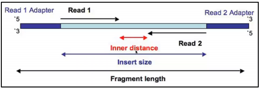
Reads can be created in two ways: single or paired. In single-end sequencing, the machine reads each DNA fragment from one end only, starting at the 5′ end and working its way across the fragment until the read is complete. In paired-end sequencing, the machine reads from both ends of the same fragment: one read starts at the 5′ end and moves toward the middle (the forward read), and the other starts at the opposite 3′ end and also moves toward the middle (the reverse read). This gives you two reads per fragment that come from opposite directions, which helps improve accuracy and recover more of the original sequence.
These reads are written to disk as plain-text files, almost always compressed and ending in .fastq.gz.
- FASTA files ( .fasta, .fa ) hold only the nucleotide characters A/T/C/G; they are mainly used once reads have been cleaned and merged (assembled).
- FASTQ files ( .fastq, .fq ) hold both the sequence and its Phred quality scores, telling you how confident the instrument was when reading each basepair of the DNA.
Once you have the downloads in place, peek inside one of the real files, say GC1GC1_R1.fastq.gz (forward reads from replicate
GC1, experimentGC1), to explore by yourself what a FASTQ record looks like and to check that the quality scores are sensible before you hand the data to QIIME 2. You can do this in bash like this:# ── Bash one-liner: show the first two reads (8 lines) ─────────── zcat /mnt/lustre/groups/WCHPC/wednesday_data/fastq/GC1GC1_R1.fastq.gz | head -n 8Breaking that command down,
zcatprints the unzipped file,head -n 8takes the top 8 lines of the file.
2 · “How many reads did I get?”
Before you begin any analysis, it’s important to check that your files actually contain the number of reads you expect. This step can catch problems like incomplete downloads, interrupted sequencing runs, or incorrect file handling.
Since each read in a FASTQ file takes up four lines (a header, sequence, separator, and quality line), you can calculate the number of reads by dividing the total number of lines by 4. This gives you a quick way to verify that your samples are complete before moving on.
## count reads in one compressed file
zcat /mnt/lustre/groups/WCHPC/wednesday_data/fastq/GC1GC1_R1.fastq.gz | wc -l | awk '{print $1/4 " reads"}'

# loop across every forward read file and list counts
for f in /mnt/lustre/groups/WCHPC/wednesday_data/fastq/*_R1.fastq.gz; do
 echo -n "$f  "
 zcat "$f" | wc -l | awk '{printf "%d reads\n",$1/4}'
done
3 · Where Is Genetic Data Stored?
Genetic data is typically stored across three main locations: local and institutional systems, high-performance computing (HPC) environments, and cloud-based storage. On local machines and institutional servers, raw sequencing outputs like .fastq.gz and .bam files are organised by project, sample, date, and run ID for easy retrieval and provenance tracking. HPC systems often employ parallel file systems such as Lustre or GPFS to store large intermediate files and QIIME 2 artifacts (.qza, .qzv), with quotas and structured directories ensuring efficient and fair use. Cloud-based storage platforms like Amazon S3 or Google Cloud Storage offer scalable solutions for ongoing projects, supporting automated dataset archiving through versioning and lifecycle policies.
Beyond private and institutional repositories, genetic data is commonly deposited in public archives to support transparency and reuse. The International Nucleotide Sequence Database Collaboration (INSDC) integrates the NCBI Sequence Read Archive (SRA), the European Nucleotide Archive (ENA), and the DNA Data Bank of Japan (DDBJ), providing global infrastructure for raw and processed sequencing data. Secondary and domain-specific archives like MG-RAST, Qiita, and Galaxy Data Libraries cater to metagenomics and microbiome studies, offering both storage and analysis pipelines. Effective data management requires integrating metadata (e.g., sample descriptors, barcodes), adhering to standard file formats (.fastq.gz, .bam, .qza/.qzv), setting access permissions, and ensuring reproducibility, for example through QIIME 2’s embedded provenance tracking.
4 · BLAST searches
If you’ve ever used BLAST (Basic Local Alignment Search Tool), you know the basic idea: you give it a DNA or protein sequence, and it compares that sequence to a reference database to find the best matches. It reports which known sequences are most similar, how long the matching region is, and how confident the match is. This is the foundation of how we assign names or functions to unknown sequences.
In amplicon analysis, tools like QIIME 2 do something very similar. After denoising your reads into amplicon sequence variants (ASVs), which are essentially cleaned-up, exact sequences, it matches each ASV to a reference database such as SILVA, Greengenes, or GTDB. Each ASV is compared to known 16S rRNA gene sequences in the database to find its closest match, which is then used to assign it a taxonomic label (e.g. Bacillus subtilis, Pseudomonas, etc.).
So while QIIME doesn’t run BLAST directly by default, it’s doing the same type of work: comparing your sequences to a trusted reference and reporting the best biological match. It’s just automated, scaled up, and optimised for microbial marker genes like 16S.
Lets run a blast search for the first sequence in our file. Print the first sequence and its information and paste it into the BLAST Nucleotide website: blast.ncbi.nlm.nih.gov/.
zcat /mnt/lustre/groups/WCHPC/wednesday_data/fastq/GC1GC1_R1.fastq.gz | head -n 4
What do you see? Is it a bacterium that you have identified? Hold onto this thought until we discuss contamination later.
Intro to HPC
High-Performance Computing (HPC) refers to the use of supercomputers or parallel computing techniques to perform complex computations quickly. HPC systems aggregate computing resources to solve problems that would be unfeasible or time-consuming using conventional methods. These systems play a critical role in research fields like bioinformatics, physics, climate modeling, and engineering.
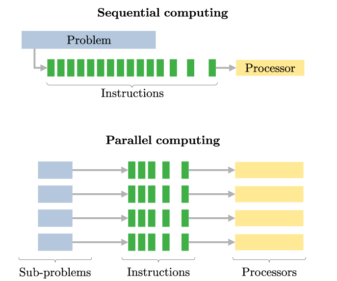
But how do HPCs achieve better results in less time? This is because of parallel computing, which is the ability to divide large tasks into smaller pieces that can be completed simultaneously. You can think of this like a group of people working together to build a house - each person has a specific task which they work on at the same time, finishing the job faster.
A frequent misunderstanding is that executing code on a cluster will automatically result in improved performance. Clusters do not inherently accelerate code execution; for enhanced performance, the code must be explicitly adapted for parallel processing, a task that falls under your responsibility as a programmer.
HPC’s typically have thousands of cores, made up by separate computers (nodes) that are linked and can transfer data to each other. The Lengau CHPC we will be using today has a total of 33,436 cores available to its users.
Qiime2 on HPC
-
CPU Power: Many QIIME2 plugins, such as dada2, vsearch, and feature-classifier, can utilize multithreading to significantly reduce processing time. On an HPC, users can request dozens of CPU cores per job, greatly accelerating large analyses involving hundreds or thousands of samples.
-
RAM Availability: Some QIIME2 steps, especially taxonomy classification and large distance matrix calculations, can consume large amounts of memory (10–100+ GB). HPC systems often provide nodes with hundreds of gigabytes of RAM, preventing crashes and memory overflows that might occur on a personal computer.
-
Storage Capacity: Intermediate QIIME2 artifacts and results (e.g., .qza, .qzv files) accumulate quickly and may exceed local storage limits. HPC environments usually offer shared high-capacity storage systems (terabytes to petabytes) optimized for fast read/write speeds, which helps manage these large datasets efficiently.
-
Job Scheduling: HPCs use job scheduling systems (e.g., SLURM, PBS) to manage and queue computational tasks. This enables long or resource-heavy QIIME2 workflows to run in the background without tying up your local machine.
Connecting to the CHPC
Much of the work we will be doing in this workshop will be on the HPC system provided by the National Integrated Cyberinfrastructure System (NICIS). This is a Linux system (so forget any Windows or Mac way of thinking!). There are 2 ways to communitcate with the CHPC:
To connect to the server, run the following command, including the username you have been assigned. This is what we will be using for the rest of the day to run our jobs:
ssh <username>@lengau.chpc.ac.za # sets up a direct connection between your computer and the CHPC.
In a separate terminal window, you can then connect and transfer files using the following command:
sftp <username>@lengau.chpc.ac.za   # sets up a secure file transfer connection between your computer and the CHPC

get <CHPC-directory> <local-directory>   # use this to get data from the CHPC and put it into a directory on your computer

put <local-directory> <CHPC-directory>   # use this to put data onto the CHPC
Setting up Anaconda3
The CHPC has a detailed explanation of setting up anaconda and python on the Lengau cluster. See here.
First we must load the necessary anaconda3 python module on the CHPC:
module load chpc/python/anaconda/3-2020.02
We will be using the packages set up in the available conda environments on the CHPC. Each time we start working with Qiime and every time we switch node, we will want to load up the environments with the following command:
conda activate /apps/chpc/bio/anaconda3-2020.02/envs/qiime2-amplicon-2024.5
To request an interactive job on the CHPC, run the following command. This will request 24 cores (an entire computing node) for 4hrs and lets you run your jobs straight into the terminal:
qsub -I -l select=1:ncpus=24:mpiprocs=24 -P WCHPC -l walltime=4:00:00
Also make a directory that you can store your outputs in:
mkdir wednesday_outputs
QIIME2
Understanding QIIME2 Files
QIIME 2 organises your analysis using two main file types: .qza files for data (called QIIME Zipped Artifacts) and .qzv files for visualisations (QIIME Zipped Visualisations). These files are more than simple containers, as they include detailed information about how each was generated, such as the input files, commands, and parameters used. This is known as provenance tracking, and it allows others to trace every step of your workflow. You can open .qzv files in your browser at https://view.qiime2.org to explore interactive summaries like quality plots, taxonomic profiles, and diversity results. This approach helps make your microbiome analysis more transparent, easier to share, and reproducible from start to finish.
Import your paired-end sequences
DNA sequencing generates data in the form of FASTQ files. Importing these files into QIIME 2 allows the software to begin processing them in a standardized format.
QIIME2 expects file locations to be written in a manifest file (here wednesday_manifest.tsv), whose internal format is specified in the --input-format. There is the option of PairedEndFastqManifestPhred33V2 or SingleEndFastqManifestPhred33V2, depending on if we supply only forward reads or paired forward-reverse reads. We would format our manifest file accordingly:
The fastq.gz absolute filepaths may contain environment variables (e.g., $HOME or $PWD). The following example illustrates a simple fastq manifest file for paired-end read data for four samples.
sample-id     forward-absolute-filepath       reverse-absolute-filepath
sample-1      $PWD/some/filepath/sample0_R1.fastq.gz  $PWD/some/filepath/sample1_R2.fastq.gz
sample-2      $PWD/some/filepath/sample2_R1.fastq.gz  $PWD/some/filepath/sample2_R2.fastq.gz
sample-3      $PWD/some/filepath/sample3_R1.fastq.gz  $PWD/some/filepath/sample3_R2.fastq.gz
sample-4      $PWD/some/filepath/sample4_R1.fastq.gz  $PWD/some/filepath/sample4_R2.fastq.gz
The following example illustrates a simple fastq manifest file for fastq single-end read data for two samples.
sample-id     absolute-filepath
sample-1      $PWD/some/filepath/sample1_R1.fastq
sample-2      $PWD/some/filepath/sample2_R1.fastq
Importing means telling QIIME where your raw data is and converting it into its internal format (when we run a command with time in front of it, it shows us how long it took to run):
time qiime tools import \
 --type 'SampleData[PairedEndSequencesWithQuality]' \
 --input-path /mnt/lustre/groups/WCHPC/wednesday_data/wednesday_manifest.tsv \
 --output-path wednesday_outputs/demux.qza \
 --input-format PairedEndFastqManifestPhred33V2
Time to run: 2 minutes
Output:
demux.qza
Examine the quality of the data
Before analyzing the sequences, it’s important to assess their quality. A quality check using QIIME2 allows us to visualize how reliable each base position is across all reads. If certain positions show low quality, we can trim them off.
Sequencers give every base a Phred quality score (Q) that converts machine‐signal strength into an error estimate. In Illumina-style short read sequencing, the machine builds each read one base at a time and each round of chemical incorporation is called a cycle. Looking at per-cycle numbers lets you spot where quality begins to drop off toward the end of the reads, and lets you set the number you wish to truncate the reads at:
| Score | Error rate | Meaning |
|---|---|---|
| Q20 | 1 error in 100 bases (99% accurate) | Acceptable but starting to get noisy |
| Q30 | 1 error in 1000 bases (99.9% accurate) | Clean data - the Illumina gold standard |
When a base falls below Q20 it can introduce false sequence variants, so we normally trim reads where Q20/Q30 statistics start to degrade.
We can view the characteristics of the dataset and the quality scores of the data by creating a QIIME2 visualization artifact.
time qiime demux summarize \
 --i-data wednesday_outputs/demux.qza \
 --o-visualization wednesday_outputs/demux.qzv
Time to run: 1 minute
Output: *
demux.qzv
This will create a visualization file. Download the file to your local computer (using sftp).
Now you can view the file on your local computer using the QIIME2 visualization server. Alternatively you can view the precomputed file on that server using the button above.
When viewing the data look for the point in the forward and reverse reads where quality scores decline below 25-30. We will need to trim reads to this point to create high quality sequence variants.
Selecting Sequence Variants
Sequencing isn’t perfect and errors, noise, and artefacts are common. To make sense of the data, the first core step is to group similar reads together and identify the true biological sequences that were present in the sample. This process is called sequence variant picking.
Modern tools like Dada2, Deblur, and UNOISE2 aim to identify these exact sequences by using statistical error correction models, taking an information theoretic approach and applying a heuristic. This is a major improvement over older methods like OTU picking, where sequences were grouped based on a similarity threshold. ASVs (Amplicon Sequence Variants) provide higher resolution, greater reproducibility, and better biological accuracy.
Sequence variant selection is the slowest step in the tutorial.
Dada2
This code will send a number every single second Dada2 is running, so that your interactive session can stay open:
(qiime dada2 denoise-paired \
 --i-demultiplexed-seqs wednesday_outputs/demux.qza \
 --o-table wednesday_outputs/table-dada2 \
 --o-representative-sequences wednesday_outputs/rep-seqs-dada2 \
 --o-denoising-stats wednesday_outputs/denoising-stats.qza \
 --p-trim-left-f 9 \
 --p-trim-left-r 9 \
 --p-trunc-len-f 220 \
 --p-trunc-len-r 200 \
 --p-n-threads 24 \
 --p-n-reads-learn 200000) & pid=$!; i=0; while kill -0 $pid 2>/dev/null; do echo $i; sleep 1; ((i++)); done; wait $pid
Time to run: 35 minutes
Output:
rep-seqs-dada2.qza: These are your representative sequences: the exact, cleaned-up ASV sequences found in your dataset. They are matched against reference databases later (like SILVA or Greengenes) to assign taxonomy.table-dada2.qzv: This is your feature table, stored in QIIME 2’s .qza format. Internally, it follows the BIOM (Biological Observation Matrix) standard. It records how many times each ASV appears in each sample, similar to a species count table. This is the key file you’ll use for diversity analysis, statistical testing, and visualisation.
Taxonomic analysis
Sequence variants (ASVs) are high-resolution markers of microbial diversity, but on their own, they don’t tell us which organisms are present. While they help define the structure of the community, we often want to go a step further and identify the actual microbes behind each sequence. To do that, we need to assign taxonomy: linking each ASV to a known group of bacteria or archaea.
This process requires two key components: a reference database of well-annotated 16S rRNA sequences, and a classification algorithm that can compare our ASVs to that database. QIIME 2 handles this automatically using pretrained classifiers. The classifier searches for the closest match in the reference and labels each ASV accordingly, down to the genus or species level if possible.
Earlier, when you ran a BLAST search on one of your raw reads, you may have seen a match to Arabidopsis thaliana. This illustrates why taxonomy assignment is more than just a formality. Host DNA, especially from chloroplasts or mitochondria, can end up in your sequences — and without a curated, microbial-only reference, those contaminants might remain in your results. By using the right database, we ensure that only relevant microbial taxa are kept for downstream analysis. The primary databases are:
| Database | Description | License |
|---|---|---|
| Silva | The most up-to-date and extensive database of prokaryotes and eukaryotes, several versions | Free academic / Paid commercial license |
| The RDP database | A large collection of archaeal bacterial and fungal sequences | CC BY-SA 3.0 |
| UNITE | The primary database for fungal ITS and 28S data | Not stated |
There are several methods of taxonomic classification available. The most commonly used classifier is the RDP classifier. Other software includes SINTAX and 16S classifier. We will be using the QIIME2’s built-in naive Bayesian classifier (which is built on Scikit-learn but similar to RDP), noting that the method, while fast and powerful, has a tendency over-classify reads.
There are two steps to taxonomic classification: training the classifier (or using a pre-trained dataset) and classifying the sequence variants. Generally it is best to train the classifier on the exact region of the 16S, 18S or ITS you sequenced.
For this tutorial we will be using a classifier model trained on the Silva 99% database trimmed to the V4 region.
time qiime feature-classifier classify-sklearn \
 --i-classifier /mnt/lustre/groups/WCHPC/wednesday_data/silva-138-99-nb-classifier.qza \
 --i-reads wednesday_outputs/rep-seqs-dada2.qza \
 --o-classification wednesday_outputs/taxonomy.qza
Time to run: 1 minute
Output:
taxonomy.qza
Create a bar plot visualization of the taxonomy data:
time qiime taxa barplot \
 --i-table wednesday_outputs/table-dada2.qza \
 --i-taxonomy wednesday_outputs/taxonomy.qza \
 --o-visualization wednesday_outputs/taxa-bar-plots.qzv
Time to run: 1 minute
Output:
taxa-bar-plots.qzv
Adding metadata and examining count tables
Once your ASV table has been generated, it needs to be connected to your sample metadata and taxonomic assignments. This step is essential for creating meaningful visual summaries and performing any ecological comparisons. Without metadata, your sequences are just anonymous counts. Metadata provides biological context — which genotype the sample comes from, which compartment (e.g. root zone, bulk soil), and which treatment it received. Taxonomy links each ASV to a known organism or group of organisms, letting us ask not just how communities vary, but who is driving that variation.
QIIME 2 allows you to integrate the count table with your mapping file to visualise how read counts distribute across samples.
qiime feature-table summarize \
 --i-table wednesday_outputs/table-dada2.qza \
 --m-sample-metadata-file /mnt/lustre/groups/WCHPC/wednesday_data/wednesday_metadata.tsv \
 --o-visualization wednesday_outputs/table-dada2.qzv
Output:
table-dada2.qzv
To visualise taxonomic composition by group or treatment:
qiime taxa barplot \
 --i-table wednesday_outputs/table-dada2.qza \
 --i-taxonomy wednesday_outputs/taxonomy.qza \
 --m-metadata-file /mnt/lustre/groups/WCHPC/wednesday_data/wednesday_metadata.tsv \
 --o-visualization wednesday_outputs/taxa-bar-plots.qzv
Output:
taxa-bar-plots.qzv
Filtering contaminants
Sequencing from soil or root material often includes host DNA like mitochondria or chloroplasts. These non-microbial sequences can obscure patterns in microbial community composition and inflate diversity estimates. Filtering out these contaminants is a standard practice in microbiome workflows, especially when studying plant-associated microbes. This helps ensure that the dataset reflects only the true microbial community of interest.
Looking at the the taxonomy.qzv file using https://view/qiime2.org We can see the data presented at different taxonomic levels and grouped by different experimental factors. If we drill down to taxonomic level 5 something looks a bit odd. There’s lots of “Rickettsiales;f__mitochondria”. This is really plant mitochondrial contamination. Some of these samples also have chloroplast contamination.
First remove unwanted taxa (like mitochondria and chloroplasts) from the ASV count table:
qiime taxa filter-table \
 --i-table wednesday_outputs/table-dada2.qza \
 --i-taxonomy wednesday_outputs/taxonomy.qza \
 --p-exclude mitochondria,chloroplast \
 --o-filtered-table wednesday_outputs/table-dada2-filtered.qza
Output:
table-dada2-filtered.qza
Then remove those same taxa from the actual DNA sequences of the ASVs, ensuring both abundance data and sequence data are clean for downstream analysis.
qiime taxa filter-seqs \
 --i-sequences wednesday_outputs/rep-seqs-dada2.qza \
 --i-taxonomy wednesday_outputs/taxonomy.qza \
 --p-exclude mitochondria,chloroplast \
 --o-filtered-sequences wednesday_outputs/rep-seqs-dada2-filtered.qza
Output:
rep-seqs-dada2-filtered.qza
Since we have altered the qza file we can create a new bar plots:
qiime taxa barplot \
 --i-table wednesday_outputs/table-dada2-filtered.qza \
 --i-taxonomy wednesday_outputs/taxonomy.qza \
 --m-metadata-file /mnt/lustre/groups/WCHPC/wednesday_data/wednesday_metadata.tsv \
 --o-visualization wednesday_outputs/taxa-bar-plots-filtered.qzv
Output:
taxa-bar-plots-filtered.qzv
Summary
Congratulations! You’ve now imported raw FASTQ sequences into QIIME 2, inspected their quality, and used DADA2 or Deblur to clean and denoise them, generating amplicon sequence variants (ASVs) and filtered organelle and host contaminants. These are a good representation of microbial diversity in your samples. You’ve produced:
- A feature table showing how many times each ASV appeared in each sample
- A list of representative ASV sequences
- A quality summary of the reads
- A taxonomic assignment of each ASV, using the SILVA database
- Bar plots that visually summarise which microbes are present in each condition
- All done having removed contaminants from your samples
Tomorrow, you’ll explore alpha and beta diversity, use ordination methods like PCoA, and run statistical tests to evaluate how microbiome composition shifts across different Arabidopsis genotypes. You’ll also learn how to export and share your results for publication or collaboration.